ANGSD: Analysis of next generation Sequencing Data
Latest tar.gz version is (0.938/0.939 on github), see Change_log for changes, and download it here.
Error estimation
ANGSD currently has 2 different methods for estimating error rates.
- A method that will estimate the joint typespecific errorrates for multiple samples. This method is using the minor allele frequency as prior, and therefore this method can not be used for single samples.
- A method that that uses an outgroup and an 'errorfree' individual. Useful for single samples.
The typespecific errorrates is an Failed to parse (SVG (MathML can be enabled via browser plugin): Invalid response ("Math extension cannot connect to Restbase.") from server "https://wikimedia.org/api/rest_v1/":): {\displaystyle 4\times 4} matrix, with the errorates of observing base A but in reality it was base C etc.
Error estimation from polymorphic sites
The method for estimating typespecific errors is described in Kim2011, and is based on the counts of the 4 different nucleotides. This method should be applied to the sites that are variable and the measure for variability is the simple MAF estimator that is described in Li2010.
- NB
The analysis will use at least numSites for that analysis. If you do not have this number of variable sites, then the analysis will not be performed.
Brief Overview
./angsd -doError
        -> angsd version: 0.564  build(Dec  6 2013 12:52:55)
        -> Analysis helpbox/synopsis information:
---------------------
analysisEstError.cpp:
-doError        0
        1: SYK method, joint typespecific errors (Multisample)
        -minSites       10000
        -errors         (null)  (Filename for starterrors)
        -emIter         100
        -minPhat        0.005000        (Minimum phat)
        -eps            0.001000        (Estimate of errorrate)
        NB this method requires -doMajorMinor 2
Options
- -numSites [int]
default 10000. This is the number of sites we want to use for this analysis.
- -cutoff [float]
default 0.005. This means we only run the error estimation on sites with a MAF>0.005. This should be modified according to the number of samples in the dataset.
- -eps [float]
default 0.001.This is a guess of the errorrate in the sample, this is used for the simple MAF estimator
- -errors [filename]
This file should contain a guess of the typespecific errors.
To further refine what data should be used please see alleles counts.
Example
The simplest example is:
./angsd -bam bam.filelist -doCounts 1 -out test -doError 1 -doMajorMinor 2 -nThreads 2 -minSites 1000
Or a more elaborate example where we only want to estimate the typespecific errors for the "good" data:
./angsd -bam bam.filelist -doCounts 1 -out test2 -doError 1 -doMajorMinor 2 -nThreads 2 -minSites 1000 -minQ 20 -minMapQ 30
Output
The output for this analysis is a file suffixed with *.error.chunkunordered.


#test
0.000000	0.005488	0.003847	0.003137\
0.006807	0.000000	0.001972	0.002396\
0.002190	0.001855	0.000000	0.008068\
0.002491	0.004268	0.005812	0.000000
#test2
0.000000	0.000071	0.003381	0.001254\
0.003989	0.000000	0.000000	0.002568\
0.002270	0.000000	0.000000	0.003650\
0.001451	0.004327	0.000974	0.000000
Notice that we for the more stringent test2 dataset have somewhat lower error rates. But we should really choose a much larger number of sites to do this analysis. Each line has 16 entries corresponding to the type specific errors for a region of -numsites.
NB Currently the ordering of each line, can not be interpreted as the error rates along the genome, due to the threading. This will likely change in future versions.
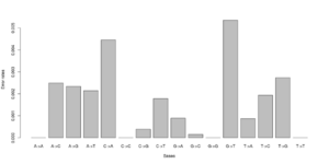
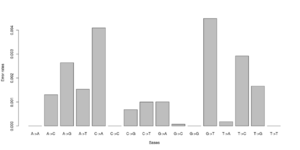
We can visualise this easily in R, see figures on right side (These are not the values from the above)
a <- as.numeric(read.table("test.error.chunkunordered",nrow=1))
b <- as.numeric(read.table("test2.error.chunkunordered",nrow=1))
DNA<-c("A","C","G","T")
names(a) <- as.vector((sapply(1:4,function(x) paste(DNA[x],DNA,sep="->"))))
barplot(a)
barplot(b)
Error estimation using an outgroup and an error free individual


The estimated rates can roughly be interpreted as relative error rates. That is excess of derived alleles in your sample compare to the derived alleles in the an error free indviduals The idea is the your sample and the error free individuals should have the same expected number of derived alleles and the extra observed derived alleles in you sample are due to the excess error. For each individual we sample a single base from the reads at each position. We use only positions were there are coverage for both the outgroup, the sample and the error free individual. See theory section below for more details.
Brief Overview
./angsd -doAncError
	-> angsd version: 0.567	 build(Dec  7 2013 14:56:25)
	-> Analysis helpbox/synopsis information:
--------------
analysisAncError.cpp:
	-doAncError	0
	1: EM v1
	2: EM v2 (Under development, don't use)
	-sample	1	(Sampling strategies, for EM v1)
	 0:	 (Use all bases)
	 1:	 (Sample single base)
	 2:	 (Sample first base)
Required:
	-ref	(null)	(fastafile containg 'perfect' sample)
	-anc	(null)	(fastafile containg outgroup)
To make matters explicit: For this analysis, the -ref should not be your reference, but a fasta file containing the consensus of a 'perfect' sample. The method will calculate the difference between the -ref and -anc, and the difference between the supplied BAM files, and interpret the excess of difference as an error. You can generate a consensus fasta with -doFasta.
Options
- -doAncError 1
Use -doAncError to use this analysis
- -anc [filename]
fasta file with the ancestral alleles
- -ref [filename]
fasta file of an error free individual.
- -sample [int]
0: Use all reads
1: Sample only one base per site (default)
2: Use first base per site
To further refine what data should be used please see alleles counts and read filters.
Example
- angsd -doAncError 1 -anc chimpHg19.fa -ref hg19perfect.fa -out results -bam bam.filelist
- Rscript R/estError.R file=results.ancError
Typing Rscript R/estError.R will give you additional options for plotting the results.
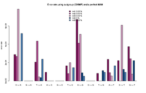
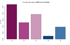
The command for plotting the figure on the right was given as:
Rscript ../angsd0.567/R/estError.R file=output/smallBamMicsAncq30Q20.ancError main="Errorrate using outgroup (CHIMP) and a perfect MAN" doPng=TRUE
- NB the script will generate an empty Rplots.pdf file. This is expected. Sorry about this. The reason is that we haven't figured out how to change the R command called palette without generating a Rplots.pdf file.
Output
- The output from the angsd cprogram is in a horrible format. Those are 2 files suffixed with *.ancError and *.ancErrorChr.
- The Rscript will output the type specific errors and the overall errors. It will also produce two figures. One will the type specific errors and one with the overall errors. If a lot of individuals are included in the analysis the figure will need to be modified. The output is 3 files: 2) figures called errorEst/errorEstOverall. And a text file containing the values used for generating the figures. Example below
"C -> A"	"G -> A"	"T -> A"	"A -> C"	"G -> C"	"T -> C"	"A -> G"	"C -> G"	"T -> G"	"A -> T"	"C -> T"	"G -> T"
"ind1"	0.000288466623749173	1e-10	0.000205229813382333	9.47513790217621e-05	1e-10	0.000165916656465779	0.000669301671751217	1e-10	8.23344455554688e-05	0.000236585677709732	0.000221600942251836	0.000373954946601755
"ind2"	0.000268442684398456	1e-10	0.000435043709474343	1e-10	1e-10	8.01698019462887e-05	0.000412983451956348	1e-10	1e-10	9.13052545304468e-05	1e-10	0.000241054281567419
"ind3"	0.000782491579122587	1e-10	4.50081140012945e-05	1.78223380523875e-06	1e-10	0.000199737488394593	0.00050873938351221	1e-10	1e-10	5.56098365280151e-05	0.000607887111412939	7.58377930673463e-05
"ind4"	1e-10	1e-10	3.74736836129833e-05	1e-10	1e-10	1e-10	8.82147055613573e-05	1e-10	0.000113908816926609	1e-10	0.000127101824285852	0.000220867678248873
"ind5"	0.00051652693307555	1e-10	0.000237392858838552	1e-10	1e-10	0.000145043068998529	5.36305888166965e-05	1e-10	9.50330440265981e-05	0.000166122730928694	9.42460521591968e-05	1e-10
"ind1 0.0538 %"
"ind2 0.0258 %"
"ind3 0.0385 %"
"ind4 0.0049 %"
"ind5 0.019 %"
Theory
These two subsection will contain the theory behind the methods.
Method 1
The method is described in kim2011 and work by simultaneously estimating allele frequencies, genotype likelihoods and the error rates.
The likelihood of the sequencing data Failed to parse (SVG (MathML can be enabled via browser plugin): Invalid response ("Math extension cannot connect to Restbase.") from server "https://wikimedia.org/api/rest_v1/":): {\displaystyle D} of Failed to parse (SVG (MathML can be enabled via browser plugin): Invalid response ("Math extension cannot connect to Restbase.") from server "https://wikimedia.org/api/rest_v1/":): {\displaystyle n} individuals for Failed to parse (SVG (MathML can be enabled via browser plugin): Invalid response ("Math extension cannot connect to Restbase.") from server "https://wikimedia.org/api/rest_v1/":): {\displaystyle M} sites can be described through the allele frequencies Failed to parse (SVG (MathML can be enabled via browser plugin): Invalid response ("Math extension cannot connect to Restbase.") from server "https://wikimedia.org/api/rest_v1/":): {\displaystyle f} and the type specific error rates Failed to parse (SVG (MathML can be enabled via browser plugin): Invalid response ("Math extension cannot connect to Restbase.") from server "https://wikimedia.org/api/rest_v1/":): {\displaystyle e}
Failed to parse (SVG (MathML can be enabled via browser plugin): Invalid response ("Math extension cannot connect to Restbase.") from server "https://wikimedia.org/api/rest_v1/":): {\displaystyle \begin{align} p(D|f,e) &= \prod_{i=1}^n \prod_{j=1}^M p(D_j^i|f_j,e)\\ &= \prod_{i=1}^n \prod_{j=1}^M \sum_{g=0}^2 p(g|f_j)p(D_j^i|g,e) \end{align}}
by summing over the unknown genotypes Failed to parse (SVG (MathML can be enabled via browser plugin): Invalid response ("Math extension cannot connect to Restbase.") from server "https://wikimedia.org/api/rest_v1/":): {\displaystyle g} . The genotype likelihood Failed to parse (SVG (MathML can be enabled via browser plugin): Invalid response ("Math extension cannot connect to Restbase.") from server "https://wikimedia.org/api/rest_v1/":): {\displaystyle p(D_j^i|g,e)} relies on the type specific error rates (see kim2011 p.14 for details). The type specific error rates are obtain along site the allele frequencies by
Failed to parse (SVG (MathML can be enabled via browser plugin): Invalid response ("Math extension cannot connect to Restbase.") from server "https://wikimedia.org/api/rest_v1/":): {\displaystyle \hat{e},\hat{f} = argmax_{f,e} p(D|f,e)}
Method 2
The method was use in Orlando2013 and is described in details in supplementary 4.4
The estimated rates can roughly be intrepreted as relative error rates. That is excess of errors in your sample compare to the error in a high quality indvidual. The idea is the your sample and the high quality individual should have the same expected number of derived alleles and the extra derived alleles in you sample are due to the excess error. We use only positions were there are coverage for both the chimp, the sample and the high quality genome. The overall error rate is obtained from
were
- Failed to parse (SVG (MathML can be enabled via browser plugin): Invalid response ("Math extension cannot connect to Restbase.") from server "https://wikimedia.org/api/rest_v1/":): {\displaystyle \epsilon} is the error rate
- Failed to parse (SVG (MathML can be enabled via browser plugin): Invalid response ("Math extension cannot connect to Restbase.") from server "https://wikimedia.org/api/rest_v1/":): {\displaystyle O_D} is the observed number of derived alleles in the sample
- Failed to parse (SVG (MathML can be enabled via browser plugin): Invalid response ("Math extension cannot connect to Restbase.") from server "https://wikimedia.org/api/rest_v1/":): {\displaystyle E_D} is the expected number of derived alleles which is obtained from the observed derived alleles from the high quality genome
- Failed to parse (SVG (MathML can be enabled via browser plugin): Invalid response ("Math extension cannot connect to Restbase.") from server "https://wikimedia.org/api/rest_v1/":): {\displaystyle E_A} is the expected number of ancestral alleles which is obtained from the high quality genome
The type specific error rates are obtained from maximizing the likehood
Failed to parse (SVG (MathML can be enabled via browser plugin): Invalid response ("Math extension cannot connect to Restbase.") from server "https://wikimedia.org/api/rest_v1/":): {\displaystyle P(H=h|D=d,e) = \prod_1^n P(H_i=h_i|D_i=d_i,e) } where n is the number of sampled bases, Failed to parse (SVG (MathML can be enabled via browser plugin): Invalid response ("Math extension cannot connect to Restbase.") from server "https://wikimedia.org/api/rest_v1/":): {\displaystyle h_i } is the observed base of the sample, Failed to parse (SVG (MathML can be enabled via browser plugin): Invalid response ("Math extension cannot connect to Restbase.") from server "https://wikimedia.org/api/rest_v1/":): {\displaystyle d_i} is the obsered base of the outgroup and e is an error rate matrix with entrance Failed to parse (SVG (MathML can be enabled via browser plugin): Invalid response ("Math extension cannot connect to Restbase.") from server "https://wikimedia.org/api/rest_v1/":): {\displaystyle e_{a->b} } being the rate of error from base a to different base b and Failed to parse (SVG (MathML can be enabled via browser plugin): Invalid response ("Math extension cannot connect to Restbase.") from server "https://wikimedia.org/api/rest_v1/":): {\displaystyle e_{a->a} } being equal to Failed to parse (SVG (MathML can be enabled via browser plugin): Invalid response ("Math extension cannot connect to Restbase.") from server "https://wikimedia.org/api/rest_v1/":): {\displaystyle 1-\sum_{b\ne a} e_{a->b}}
We calculate the above by summing over the true unobserved base Failed to parse (SVG (MathML can be enabled via browser plugin): Invalid response ("Math extension cannot connect to Restbase.") from server "https://wikimedia.org/api/rest_v1/":): {\displaystyle T_{i} } Failed to parse (SVG (MathML can be enabled via browser plugin): Invalid response ("Math extension cannot connect to Restbase.") from server "https://wikimedia.org/api/rest_v1/":): {\displaystyle \begin{align} P(H_i=h_i|D_i=d_i,e) &= \sum_{t_i\in\{A,C,G,T,\}} P(H_i=h_i,T_i=t_i|D_i=d_i,e) \\ &= \sum_{t_i\in\{A,C,G,T,\}} P(H_i=h_i|T_i=t_i,e)P(T_i=t_i|D_i=d_i) \\ &= \sum_{t_i\in\{A,C,G,T,\}} e_{t_i->h_i}P(T_i=t_i|D_i=d_i) \end{align} }
Failed to parse (SVG (MathML can be enabled via browser plugin): Invalid response ("Math extension cannot connect to Restbase.") from server "https://wikimedia.org/api/rest_v1/":): {\displaystyle P(T_i=t_i|D_i=d_i) }
is set equal to the observed fraction of sites in the high quality genome where the outgroup has base Failed to parse (SVG (MathML can be enabled via browser plugin): Invalid response ("Math extension cannot connect to Restbase.") from server "https://wikimedia.org/api/rest_v1/":): {\displaystyle d_i}
and the high qualtiy genome has base Failed to parse (SVG (MathML can be enabled via browser plugin): Invalid response ("Math extension cannot connect to Restbase.") from server "https://wikimedia.org/api/rest_v1/":): {\displaystyle t_i}
