ANGSD: Analysis of next generation Sequencing Data
Latest tar.gz version is (0.938/0.939 on github), see Change_log for changes, and download it here.
SFS Estimation: Difference between revisions
No edit summary |
|||
| Line 58: | Line 58: | ||
=Brief Overview= | =Brief Overview= | ||
<pre> | <pre> | ||
./angsd - | ./angsd -dosaf | ||
-> angsd version: 0.935-44-g02a07fc-dirty (htslib: 1.12-1-g9672589) build(Jul 8 2021 08:04:55) | |||
-> ./angsd -dosaf | |||
-> Analysis helpbox/synopsis information: | |||
-> Wed Aug 18 11:09:03 2021 | |||
-> doMcall=0 | |||
-------------- | -------------- | ||
abcSaf.cpp: | abcSaf.cpp: | ||
-doSaf 0 | |||
1: perform multisample GL estimation | |||
2: use an inbreeding version | |||
3: calculate genotype probabilities (use -doPost 3 instead) | |||
4: Assume genotype posteriors as input (still beta) | |||
-underFlowProtect 0 | |||
-anc (null) (ancestral fasta) | |||
-noTrans 0 (remove transitions) | |||
-pest (null) (prior SFS) | |||
-isHap 0 (is haploid beta!) | |||
-doPost 0 (doPost 3,used for accesing saf based variables) | |||
NB: | NB: | ||
If -pest is supplied in addition to -doSaf then the output will then be posterior probability of the sample allelefrequency for each site | |||
</pre> | </pre> | ||
Revision as of 11:10, 18 August 2021
Latest version can now do bootstrapping. Folding should now be done in realSFS and not in the saf file generation.
Quick Start
The process of estimating the SFS and multidimensional has improved a lot in the newer versions.
Assuming you have a bam/cram file list in the file 'file.list' and you have your ancestral state in ancestral.fasta, then the process is:
#no filtering
./angsd -gl 1 -anc ancestral -dosaf 1
#or alot of filtering
./angsd -gl 1 -anc ancestral -dosaf 1 -baq 1 -C 50 -minMapQ 30 -minQ 20

#this will generate 3 files
1) angsdput.saf.idx 2) angsdput.saf.pos.gz 3) angsdput.saf.gz
#these are binary files that are formally defined in https://github.com/ANGSD/angsd/blob/newsaf/doc/formats.pdf

#To find the global SFS based on the run from above simply do
./realSFS angsdput.saf.idx
##or only use chromosome 22
./realSFS angsdput.saf.idx -r 22

## or specific regions
./realSFS angsdput.saf.idx -r 22:100000-150000000

##or limit to a fixed number of sites
./realSFS angsdput.saf.idx -r 17 -nSites 10000000

##or you can find the 2dim sf by
./realSFS ceu.saf.idx yri.saf.idx
##NB the program will find the intersect internally. No need for multiple runs with angsd main program.

##or you can find the 3dim sf by
./realSFS ceu.saf.idx yri.saf.idx MEX.saf.idx
SFS
This method will estimate the site frequency spectrum, the method is described in Nielsen2012. The theory behind the model is briefly described here
This is a 2 step procedure first generate a ".saf" file (site allele frequency likelihood), followed by an optimization of the .saf file which will estimate the Site frequency spectrum (SFS).
For the optimization we have implemented 2 different approaches both found in the misc folder. The diagram below shows the how the method goes from raw bam files to the SFS.
You can also estimate a 2dsfs or even higher if you want to.
* NB the ancestral state needs to be supplied for the full SFS, but you can use the -fold 1 to estimate the folded SFS and then use the reference as ancestral.
* NB the output from the -doSaf 2 are not sample allele frequency likelihoods but sample alle posteriors.
And applying the realSFS to this output is therefore NOT the ML estimate of the SFS as described in the Nielsen 2012 paper,
but the 'Incorporating deviations from Hardy-Weinberg Equilibrium (HWE)' section of that paper.
<classdiagram type="dir:LR">
[sequence data{bg:orange}]->GL[genotype likelihoods|SAMtools;GATK;SOAPsnp;Kim et.al]
[genotype likelihoods|SAMtools;GATK;SOAPsnp;Kim et.al]->doSaf[.saf file{bg:blue}] [.saf file{bg:blue}]->optimize('realSFS')[.saf.ml file{bg:red}]
</classdiagram>
Brief Overview
./angsd -dosaf
	-> angsd version: 0.935-44-g02a07fc-dirty (htslib: 1.12-1-g9672589) build(Jul  8 2021 08:04:55)
	-> ./angsd -dosaf
	-> Analysis helpbox/synopsis information:
	-> Wed Aug 18 11:09:03 2021
	-> doMcall=0
--------------
abcSaf.cpp:
	-doSaf		0
	1: perform multisample GL estimation
	2: use an inbreeding version
	3: calculate genotype probabilities (use -doPost 3 instead)
	4: Assume genotype posteriors as input (still beta)
	-underFlowProtect	0
	-anc			(null) (ancestral fasta)
	-noTrans		0 (remove transitions)
	-pest			(null) (prior SFS)
	-isHap			0 (is haploid beta!)
	-doPost			0 (doPost 3,used for accesing saf based variables)
NB:
	  If -pest is supplied in addition to -doSaf then the output will then be posterior probability of the sample allelefrequency for each site
misc/realSFS
./realSFS afile.saf.idx [-start FNAME -P nThreads -tole tole -maxIter  -nSites ]
For information and parameters concerning the realSFS subprogram go here: realSFS
Options
- -doSaf 1
- Calculate the Site allele frequency likelihood based on individual genotype likelihoods assuming HWE
- -doSaf 2
- (version above 0.503) Calculate per site posterior probabilities of the site allele frequencies based on individual genotype likelihoods while taking into account individual inbreeding coefficients. This is implemented by Filipe G. Vieira. You need to supply a file containing all the inbreeding coefficients. -indF. Consider if you want to either get the MAP estimate by using all sites, or get the standardized values by conditioning on the called snpsites. See bottom of this page for examples.
- -doSaf 3
- Calculate the genotype posterior probabilities for all samples forall sites, using an estimate of the sfs (sample allele frequency distribution). This needs a prior distribution of the SFS (which can be obtained from -doSaf 1/realSFS).
- -doSaf 4
- Calculate the posterior probabilities of the sample allele frequency distribution for each site based on genotype probabilities. The genotype probabilities should be provided by the using using the -beagle options. Often the genotype probabilities will be obtained by haplotype imputation.
- -underFlowProtect [INT]
0: (default) no underflow protection. 1: use underflow protection. For large data sets (large number of individuals) underflow projection is needed.
Output file
The output file from the -doSaf is described in detail in angsd/doc/formats.pdf. These binary annoying files can be printed with
realSFS print myfile.saf.idx
#or
realSFS print mayflies.saf.idx -r chr1:10000-20000
Example
A full example is shown below where we use the test data that can be found on the quick start page. In this example we use GATK genotype likelihoods.
first generate .saf file with 4 threads
./angsd -bam bam.filelist -doSaf 1 -out small -anc chimpHg19.fa -GL 2 -P 4
We always recommend that you filter out the bad qscore bases and meaningless mapQ reads. eg -minMapQ 1 -minQ 20. So the above analysis with these filters can be written as:
./angsd -bam bam.filelist -doSaf 1 -out small -anc chimpHg19.fa -GL 2 -P 4 -minMapQ 1 -minQ 20
Obtain a maximum likelihood estimate of the SFS using EM algorithm
misc/realSFS small.saf.idx -maxIter 100 -P 4 >small.sfs

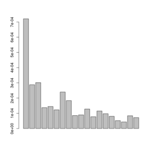
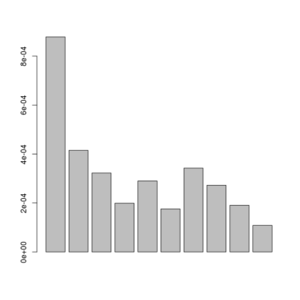
A plot of this figure are seen on the right. The jaggedness is due to the very low number of sites in this small dataset.
Interpretation of the output file
Each row is a region of the genome (see below). Each row is the expected values of the SFS.
NB
The generation of the .saf file contains a saf for each site, whereas the optimization requires information for a region of the genome. The optimization will therefore use large amounts of memory.
Folded spectra
If you don't have the ancestral state, you can instead estimate the folded SFS. This is done by supplying the -anc with the reference genome and applying -fold 1 to realSFS.
The above example would then be
#first generate .saf file
./angsd -bam bam.filelist -doSaf 1 -out smallFolded -anc  chimpHg19.fa -GL 2
#now try the EM optimization with 4 threads
misc/realSFS smallFolded.saf.idx -maxIter 100 -P 4 >smallFolded.sfs
#in R
sfs<-scan("smallFolded.sfs")
barplot(sfs[-1])

Posterior of the per-site distributions of the sample allele frequency
If you supply a prior for the SFS (which can be obtained from the -doSaf/realSFS analysis), the output of the .saf file will no longer be site allele frequency likelihoods but instead will be the log posterior probability of the sample allele frequency for each site in logspace.
Format specification of binary .saf* files
This can be found in the angsd/doc/formats.pdf
- If the -fold 1 has been set, then the dimension is no longer 2*nInd+1 but nInd+1 (this is deprecated)
- If the -pest parameter has been supplied the output is no longer likelihoods but log posterior site allele frequencies
Bootstrapping
We have recently added the possibility to bootstrap the SFS. Which can be very usefull for getting confidence intervals of the estimated SFS.
This is done by:
realSFS pop.saf.idx -bootstrap 100 -P number_of_cores
The program will then get you 100 estimates of SFS, based on data that has been subsampled with replacement.
How to plot
Assuming the we have obtained a single global sfs(only one line in the output) from realSFS program, and this is located in file.saf.sfs, then we can plot the results simply like:
sfs<-(scan("small.sfs")) #read in the log sfs
barplot(sfs[-c(1,length(sfs))]) #plot variable sites

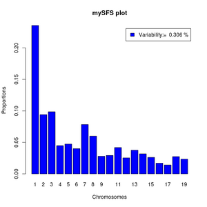
We can make it more fancy like below:
#function to normalize
norm <- function(x) x/sum(x)
#read data
sfs <- (scan("small.sfs"))
#the variability as percentile
pvar<- (1-sfs[1]-sfs[length(sfs)])*100
#the variable categories of the sfs
sfs<-norm(sfs[-c(1,length(sfs))])
barplot(sfs,legend=paste("Variability:= ",round(pvar,3),"%"),xlab="Chromosomes",
names=1:length(sfs),ylab="Proportions",main="mySFS plot",col='blue')

If your output from realSFS contains more than one line, it is because you have estimated multiple local SFS's. Then you can't use the above commands directly but should first pick a specific row.
sfs<-(as.numeric(read.table("multiple.sfs")[1,])) #first region.
#do the above
sfs<-(as.numeric(read.table("multiple.sfs")[2,])) #second region.
Which genotype likelihood model should I choose ?
It depends on the data. As shown on this example Glcomparison, there was a huge difference between -GL 1 and -GL 2 for older 1000genomes BAM files, but little difference for newer bam files.
Validation
The validation is based on the pre 0.900 version
-doSaf 1
cd misc;
./supersim -outfiles test -npop 1 -nind 12 -pvar 0.9 -nsites 50000
echo testchr1 100000 >test.fai
../angsd -fai test.fai -glf test.glf.gz -nind 12 -doSaf 1 -issim 1
./realSFS angsdput.saf 24 2>/dev/null >res
cat res
31465.429798 4938.453115 2568.586388 1661.227445 1168.891114 975.302535 794.727537 632.691896 648.223566 546.293853 487.936192 417.178505 396.200026 409.813797 308.434836 371.699254 245.585920 322.293532 282.980046 292.584975 212.845183 196.682483 221.802128 236.221205 197.914673
-doSaf 2
ngsSim=../ngsSim/ngsSim
angsd=./angsd
realSFS=./misc/realSFS

$ngsSim  -npop 1 -nind 24 -nsites 1000000 -depth 4 -F 0.0 -outfiles testF0.0
$ngsSim  -npop 1 -nind 24 -nsites 1000000 -depth 4 -F 0.9 -outfiles testF0.9

for i in `seq 24`;do echo 0.9;done >indF
echo testchr1 250000000 >test.fai
$angsd -fai test.fai -issim 1 -glf testF0.0.glf.gz -nind 24 -out noF -dosaf 1
$angsd -fai test.fai -issim 1 -glf testF0.9.glf.gz -nind 24 -out withF -dosaf 2 -domajorminor 1 -domaf 1 -indF indF
$angsd -fai test.fai -issim 1 -glf testF0.9.glf.gz -nind 24 -out withFsnp -dosaf 2 -domajorminor 1 -domaf 1 -indF indF -snp_pval 1e-4

$realSFS noF.saf 48 >noF.sfs
$realSFS withF.saf 48 >withF.sfs


#in R
trueNoF<-scan("testF0.0.frq")
trueWithF<-scan("testF0.9.frq")
pdf("sfsFcomparison.pdf",width=14)
par(mfrow=c(1,2),width=14)
barplot(trueNoF[-1],main='true sfs F=0.0')
barplot(trueWithF[-1],main='true sfs F=0.9')

estWithF<-scan("withF.sfs")
estNoF<-scan("noF.sfs")


barplot(rbind(trueNoF,estNoF)[,-1],main="true vs est SFS F=0 (ML) (all sites)",be=T,col=1:2)
barplot(rbind(trueWithF,estWithF)[,-1],main='true vs est sfs=0.9 (MAP) (all sites)',be=T,col=1:2)

readBjoint <- function(file=NULL,nind=10,nsites=10){
  ff <- gzfile(file,"rb")
  m<-matrix(readBin(ff,double(),(2*nind+1)*nsites),ncol=(2*nind+1),byrow=TRUE)
  close(ff)
  return(m)
}


m <- exp(readBjoint("withF.saf",nind=24,5e6))
barplot(rbind(trueWithF,colMeans(m))[,-1],main='true vs est sfs F=0.9 (colmean of site pp) (all sites)',be=T,col=1:2)
m <- exp(readBjoint("withFsnp.saf",nind=24,5e6))
m <- colMeans(m)*nrow(m)
##m contains SFS for absolute frequencies
m[1] <-1e6-sum(m[-1])
##m now contains a corrected estimate containing the zero category
barplot(rbind(trueWithF,norm(m))[,-1],main='true vs est sfs F=0.9 (colmean of site pp) (called snp sites)',be=T,col=1:2)

dev.off()
See results from above here:http://www.popgen.dk/angsd/sfsFcomparison.pdf
safv3 comparison
Between 0.800 and 0.900 i decided to move to a better format than the raw sad files. This new format takes up half the storage and allows for easy random access and generalizes to unto 5dimensional sfs. A comparison can be found here: safv3
Using NGStools
See realSFS for how to convert the new safformat to the old safformat if you use NGStools.