CATS
Jump to navigation
Jump to search
joint power of a non-symetric two stage GWA design
R package for power estimation for a two-stage genome-wide association design. This is a modification of the code from Skol et al 2006, nat genet. so that the relative risk, case-control ratios and allele frequencies are allowed to vary between stages.
cite
Skol, AD, Scott, LJ, Abecasis, GR, Boehnke, M (2006). Joint analysis is more efficient than replication-based analysis for two-stage genome-wide association studies. Nat. Genet., 38, 2:209-13.
Download and installation
This package only seems to work on linux.
install R package from command line
wget http://popgen.dk/software/download/CATS/CATS_1.02.tar.gz
R CMD INSTALL CATS_1.02.tar.gz
run in R
library(CATS)
cats(freq=0.2,ncases=500,ncases2=500,ncontrols=1000,ncontrols2=1000,risk=1.5,multiplicative=1)


Expected Power is;
                   For a one-stage study = 0.94
      For first stage in two-stage study = 0.972
For second stage in replication analysis = 0.784
    For second stage in a joint analysis = 0.929
                                      pi = 0.5
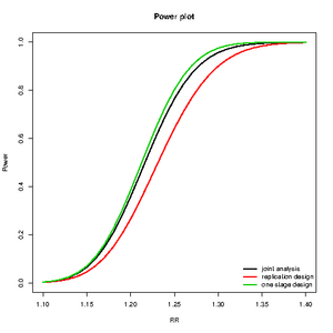
plot examples
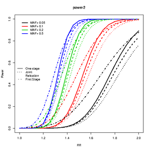
Which design is better

library(CATS)
rr<-seq(1,2,by=0.05)
maf<-c(0.05,0.1,0.2,0.5)
c2<-curve.cats(rr,maf,ncases=600,ncontrols=600,ncases2=600,
ncontrols2=600,alpha=0.000001,prevalence=0.01);

plot(c2,type="One",main="power2",ylab="Power",xlab="RR",file=NULL,col=1:4)
lines.cats(c2,type="Replication",lty=3)
lines.cats(c2,type="Joint",lty=2)
lines.cats(c2,type="First",lty=4)
legend("left",c("One stage","Joint","Relication","First Stage"),lty=1:4,bty="n")
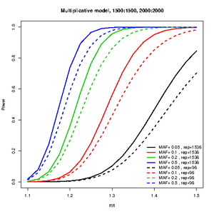
Number of SNPs for replication

library(CATS)
     power.J96<-c()
     power.J1536<-c()
     RR<-seq(1.1,1.5,by=0.025)


     maf=c(5,10,20,50)/100

for(tal2 in 1:length(maf)){
     J1<-c()
     J2<-c()
     for(tal in 1:length(RR)){
       temp<-cats(freq=maf[tal2],ncases=1500,ncontrols=1500,ncases2=2000,
ncontrols2=2000,risk=RR[tal],pimarkers = 96/300000,alpha=0.05/300000)
       J1[tal]<-temp$P.joint
       temp<-cats(freq=maf[tal2],ncases=1500,ncontrols=1500,ncases2=2000,
ncontrols2=2000,risk=RR[tal],pimarkers = 1536/300000,alpha=0.05/300000)
       J2[tal]<-temp$P.joint
     }
  power.J96<-cbind(power.J96,J1)
  power.J1536<-cbind(power.J1536,J2)

}
col=1:length(maf)

plot(RR,power.J1536[,1],type=type,lwd=2,ylab="Power",main="Multiplicative model,
 1500:1500, 2000:2000",col=col[1],ylim=0:1)
for(tal2 in 2:length(maf)){
     lines(RR,power.J1536[,tal2],lwd=2,col=col[tal2],type=type)
}
for(tal2 in 1:length(maf)){
     lines(RR,power.J96[,tal2],lwd=2,col=col[tal2],type=type,lty=2)
}
      legend("bottomright",c(paste("MAF=",c(maf),", rep=1536"),paste("MAF=",c(maf),", rep=96")),col=col,lwd=2,bty="n",lty=c(rep(1,length(maf)),rep(2,length(maf))))
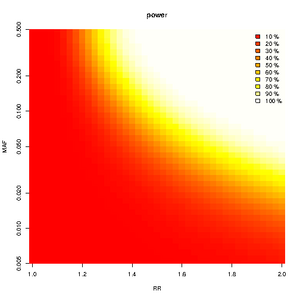
heatmap of power

library(CATS)
rr<-seq(1,2,by=0.025)
c<-super.cats(rr,by=length(rr),ncases=765,ncontrols=1274,ncases2=100,ncontrols2=100,
alpha=0.001,prevalence=0.01);

plot(c,main="power",file=NULL)
design and MAF

library(CATS)
rr<-seq(1,2,by=0.05)
maf<-c(0.05,0.1,0.2,0.5)
c2<-curve.cats(rr,maf,ncases=600,ncontrols=600,ncases2=600,ncontrols2=600,
alpha=0.000001,prevalence=0.01);

plot(c2,type="One",main="power2",ylab="Power",xlab="RR",file=NULL,col=1:4)
lines.cats(c2,type="Replication",lty=3)
lines.cats(c2,type="Joint",lty=2)
lines.cats(c2,type="First",lty=4)
legend("left",c("One stage","Joint","Relication","First Stage"),lty=1:4,bty="n")